

관련 글 목록
1. 들어가며
이번 글에서는 자산배분전략의 벤치마크로 주로 활용되는 60/40 포트폴리오를 살펴보려고 한다. 60/40 포트폴리오는 자산의 60%를 주식에 나머지 40%를 채권에 배분하는 전략이다. 이전 글에서 다루었던 유대인 전략은 자산을 3등분하는 동일가중 포트폴리오 전략이었지만 이 전략은 자산군간 비중을 다르게 가져가는 포트폴리오 전략이다. 이번 글에서는 60/40 포트폴리오의 백테스팅 결과를 살펴보고, 주식:채권 비중을 다르게 가져갔을 때 성과 지표들이 어떻게 달라지는지 확인해보려고 한다.
2. 60/40 포트폴리오 백테스팅
거인의 포트폴리오(강환국) p.155-p.161
| 투자전략 | 60/40 포트폴리오 |
| 기대 연복리수익률 | 8% 전후 |
| 포함자산 | 미국주식(SPY), 미국 중기국채(IEF) |
| 매수전략 | SPY에 60%, IEF에 40% 투자 |
| 매도전략 | 연 1회 리밸런싱 |
60/40 포트폴리오의 주요 지표(1970.1~2021.8)
| 포트폴리오 | 초기자산 (달러) |
최종자산 (달러) |
연복리 수익률(%) |
표준편자 (%) |
수익 난 월 (%) |
MDD (%) |
샤프비율 |
| 60/40 포트폴리오 |
10,000 | 1,252,954 | 9.8 | 9.8 | 64.7 | -29.5 | 0.52 |
<거인의 포트폴리오>에 제시된 60/40 포트폴리오의 백테스팅 결과는 위와 같다. 이 결과도 이전 글에서 설명한 것과 마찬가지로 Allocate smartly에서 가져온 것으로 보인다.
import pandas as pd
import numpy as np
from matplotlib import pyplot as plt
IPython_default = plt.rcParams.copy()
plt.style.use('tableau-colorblind10')

import yfinance as yf
import pyfolio as pf

tickers = ['SPY', 'IEF']
df_close = yf.download(tickers=tickers,
                 period='max',
                 interval='1d',
                 auto_adjust=True # True: adjust all OHLC automatically
                 )['Close'][tickers]

weights = [0.6, 0.4]

print('Start date of each stock')
print('-'*25)
for ticker in tickers:
    print(f"{ticker}: {df_close[[ticker]].dropna().iloc[0].name.strftime('%Y-%m-%d')}")
print('-'*25)

Start date of each stock
-------------------------
SPY: 1993-01-29
IEF: 2002-07-30
-------------------------
SPY의 데이터는 1993년 1월 29일부터 있고, IEF 데이터는 2002년 7월 30일부터 있다. Allocate Smartly의 방식과 유사하게 ETF의 벤치마크 인덱스(benchmark index)를 가져와서 1970년 ~ ETF 상장일 전 시점까지의 데이터를 만들어보려고 했는데, IEF의 벤치마크 인덱스인 ICE US Treasury 7-10 Year Index와 IEF의 괴리율이 크게 나타났다. ICE US Tresury 7-10 Year Index는 야후 파이낸스에 데이터가 없어서 FRED에 있는 데이터를 가져와서 비교해보았다.
df_IEF = yf.download(tickers=['IEF'],
                     period='max',
                     interval='1d',
                     back_adjust=False,
                     auto_adjust=False # True: adjust all OHLC automatically
                     )[['Close']]

df_IEF.columns = ['IEF']

import pandas_datareader.data as web
df_IEF_index = web.DataReader('BAMLCC4A0710YTRIV', 'fred', start='1992-06-30')
df_IEF_index.columns = ['ICE US Treasury 7-10 Year Index']

df = pd.concat([df_IEF, df_IEF_index], axis=1).dropna()
df = df/df.iloc[0]

df.plot(figsize=(12, 8));
ishares 홈페이지에서 IEF에 대한 설명을 보면 벤치마크 인덱스가 여러 번 변경된 것으로 나오는데, 이것 때문에 차이가 큰 것인지는 정확하게 확인하지 못했다(Barclays U.S. 7-10 Year Treasury Bond Index의 과거 데이터를 확인할 수 있는 곳을 찾지 못함).
iShares 7-10 Year Treasury Bond ETF | IEF
The Hypothetical Growth of $10,000 chart reflects a hypothetical $10,000 investment and assumes reinvestment of dividends and capital gains. Fund expenses, including management fees and other expenses were deducted. The performance quoted represents past p
www.ishares.com
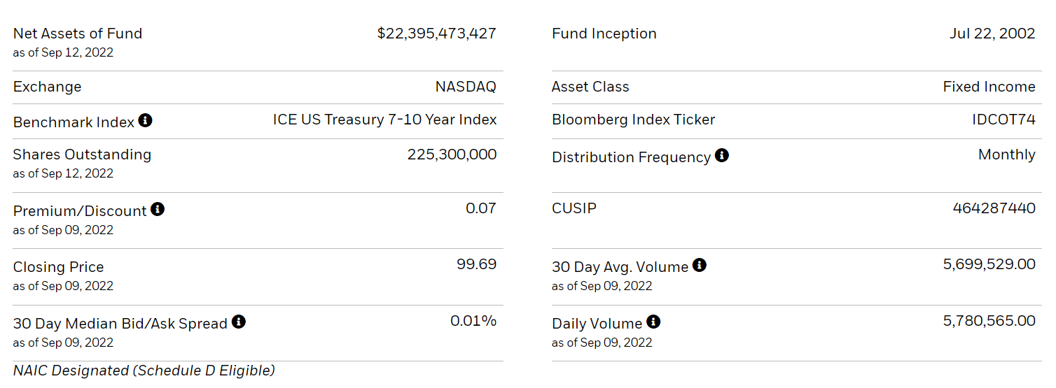
On 3/1/2021 IEF began to track the 4pm pricing variant of the ICE US Treasury 7-10 Year Index. Index data on and after 3/1/2021 is for the 4pm pricing variant of the ICE US Treasury 7-10 Year Index. Historical index data from 4/1/2016 through 2/28/2021 is for the 3pm pricing variant of the ICE US Treasury 7-10 Year Index. In order to facilitate the transition from the 3pm pricing variant to the 4pm pricing variant, historical index data for 3/1/2021 includes an additional hour of performance from 3-4pm on 2/26/2021, which accounts for 46 basis points of performance, as calculated by the index provider. A basis point is one hundredth of one percent. Historical index data prior to 4/1/2016 is for the Barclays U.S. 7-10 Year Treasury Bond Index.
Allocate Smartly에서는 아마 벤치마크 인덱스에 대한 정확한 과거 데이터를 가져와서 simulated data를 만들었을 것 같은데, 개인 투자자 수준에서 그 데이터를 구하는 게 쉽지는 않아 보인다(그냥 내가 못찾은 걸 수도 있다.). 일단 사용 가능한 데이터만 가지고 백테스팅을 진행해보았다.
df = df_close.dropna()

"""
define trading period

time_period: dataframe converted from datetime index of price dataframe
traiding_period: dataframe contains start_date and end_date of trading
 + resampled from time_period to yearly frequency and last business day of a month
 + last day of time_period assigned to last end_date
"""
time_period = df.index.to_frame()
trading_period = time_period.resample('BM').last().iloc[::12, :].rename(columns={'Date':'start_date'})
trading_period = trading_period.assign(end_date=trading_period.start_date.shift(-1).fillna(time_period.iloc[-1].name))
trading_period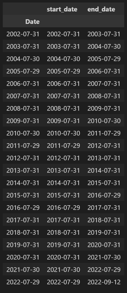
def get_mdd(df_price, start, end, col):
    """
    generates maximum drawdown(MDD) of asset prices
    MDD: the maximum observed loss from a peak to a trough of a portfolio, before a new peak is attained

    Parameters
    ----------
    df_price: pd.DataFrame
        dataFrame with datetime index and (adjusted) close prices

        example:
        ----------------------------------------------------
                    SPY	        IEF
        Date
        2002-07-30	61.6628	    46.0411
        2002-07-31	61.8120	    46.4633
        ...	        ...	        ...
        2022-09-15	388.5240	98.6000
        2022-09-16	385.5600	98.6800
        ----------------------------------------------------

    start: datetime
        trading start date
        example: Timestamp('2004-11-30 00:00:00')

    end: datetime
        trading end date
        example: Timestamp('2005-11-30 00:00:00')

    col: str
        The column name of the cumulative return of the asset for which MDD is to be calculated

    Return
    ----------
    return: pd.Series
        Series of MDD for the trading period
    """

    # select data within the trading period
    df_price = df_price[start:end].copy()

    return ((df_price[col]-df_price[col].cummax())/df_price[col].cummax()).cummin()

def get_pf_returns(df_price, tickers, start, end, weights=None, use_signal=None):
    """
    generates portfolio returns

    Parameters
    ----------
    df_price: pd.DataFrame
        dataFrame with datetime index and (adjusted) close prices
        example:
        ----------------------------------------------------
                    SPY	        IEF
        Date
        2002-07-30	61.6628	    46.0411
        2002-07-31	61.8120	    46.4633
        ...	        ...	        ...
        2022-09-15	388.5240	98.6000
        2022-09-16	385.5600	98.6800
        ----------------------------------------------------

    tickers: list
        list of tickers
        example: ['SPY', 'IEF']

    start: datetime
        trading start date
        example: Timestamp('2004-11-30 00:00:00')

    end: datetime
        trading end date
        example: Timestamp('2005-11-30 00:00:00')

    weights: list, optional
        list of weights. if weights is None, equal weights are assumed
        example: [0.6, 0.4]

    use_signal: Boolean, optional
        True/False. if True is assigned, buy signal is used. #### future work

    Return
    ----------
    return: pd.DataFrame
        prices, daily returns, cumulative returns, MDD for each asset and the portfolio
    example:
    ----------------------------------------------------
            SPY	IEF	SPY_RET	IEF_RET	PF_RET	SPY_CUMRET	IEF_CUMRET	PF_CUMRET	SPY_MDD	IEF_MDD	PF_MDD
    Date
    2002-07-31	0.0000	0.0000	0.0000	0.0000	0.0000	1.0000	1.0000	1.0000	0.0000	0.0000	0.0000
    2002-08-01	60.1982	46.6548	-0.0261	0.0041	-0.0110	0.9739	1.0041	0.9890	-0.0261	0.0000	-0.0110
    2002-08-02	58.8489	47.0152	-0.0224	0.0077	-0.0073	0.9521	1.0119	0.9817	-0.0479	0.0000	-0.0183
    ...	...	...	...	...	...	...	...	...	...	...	...
    2003-07-30	68.3896	49.3867	-0.0024	0.0080	0.0028	1.1064	1.0629	1.0959	-0.1886	-0.0743	-0.0733
    2003-07-31	68.5482	49.0572	0.0023	-0.0067	-0.0022	1.1090	1.0558	1.0936	-0.1886	-0.0743	-0.0733
    ----------------------------------------------------
    """
    # define weights
    if weights is None:
        weights = [1/len(tickers) for _ in range(len(tickers))]

    # calculate daily returns
    ret_dict = {f'{ticker}'+'_RET': df_price[ticker].pct_change().fillna(0) for ticker in tickers}
    df_price = df_price.assign(**ret_dict)

    # select data within the trading period
    df_trade = df_price.loc[start:end].copy()

    # assign 0 for the first row. returns cannot be calculated on the first trading day
    df_trade.loc[start, :] = 0

    #### future work
    """
    if use_signal==True:
        df_sig = pd.concat([df_trade.index.to_frame().drop(columns=['Date']),
                            df.loc[[start], sig_dict.keys()]
                           ], axis=1).ffill()
        df_sig.columns = tickers
        df_trade = df_trade.assign(**{col: df_trade[col]*df_sig[col] for col in tickers})
    else:
        df_trade = df_trade.assign(**{col: df_trade[col] for col in tickers})
    """

    # calculate daily portfolio returns
    df_trade = df_trade.assign(PF_RET=df_trade[ret_dict.keys()].dot(weights))

    # calculate cumulative returns within the trading period
    cumret_dict = {f'{col}_CUMRET': (1+df_trade[f'{col}_RET']).cumprod() for col in tickers}
    df_trade = df_trade.assign(PF_RET=df_trade[ret_dict.keys()].dot(weights),
                               **cumret_dict,
                               PF_CUMRET=(1+df_trade[ret_dict.keys()].dot(weights)).cumprod())
    cumret_cols = [col for col in df_trade.columns if 'CUMRET' in col]

    # calculate MDD within the trading period
    mdd_dict = {col.split('_')[0]+'_MDD': get_mdd(df_price=df_trade,
                                                  start=df_trade.index[0],
                                                  end=df_trade.index[-1],
                                                  col=col)
                                                  for col in cumret_cols}
    df_trade = df_trade.assign(**mdd_dict)

    return df_trade
df_res = pd.DataFrame()
for i in range(len(trading_period)):
df_trade = get_pf_returns(df_price=df,
tickers=tickers,
start=trading_period.iloc[i].start_date,
end=trading_period.iloc[i].end_date
)
df_res = pd.concat([df_res, df_trade], axis=0)
"""
drop duplicated rows of trading result dataframe
there are duplicated rows for each trading period except the first
"""
df_res = df_res.reset_index().drop_duplicates(['Date'], keep='first').set_index('Date')plt.rcParams.update(IPython_default);
plt.style.use('_mpl-gallery')
(1+df_res[['SPY_RET', 'IEF_RET', 'PF_RET']]).cumprod().plot(figsize=(12,8), linewidth=1)
plt.title('Cumulative returns')
plt.tight_layout();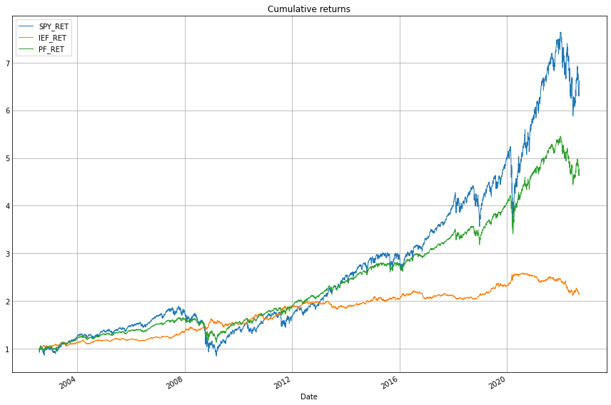
이전 글에서는 pyfolio의 함수 중 create_return_tear_sheet을 사용했었는데, 패키지 API를 좀 살펴보니 성과 지표 테이블과 그래프들을 추출하는 함수들이 각각 존재했다. 성과 지표 테이블은 show_perf_stats 함수를 이용하면 추출할 수 있다.
pf.show_perf_stats(returns=df_res.PF_RET)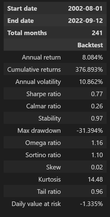
60/40 포트폴리오의 주요 지표(1970.1~2021.8)
| 포트폴리오 | 초기자산 (달러) |
최종자산 (달러) |
연복리 수익률(%) |
표준편자 (%) |
수익 난 월 (%) |
MDD (%) |
샤프비율 |
| 60/40 포트폴리오 |
10,000 | 1,252,954 | 9.8 | 9.8 | 64.7 | -29.5 | 0.52 |
Allocate Smartly에서 60/40 포트폴리오의 백테스트 결과는 무료로 확인할 수 있어서 결과값을 가져와보았다.
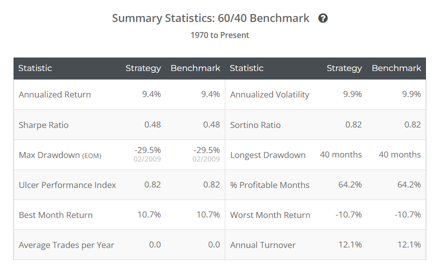
1970년~2001년 데이터를 포함했을 때와 비교해보면 연복리수익률(Annual return)의 차이가 꽤 크게 나타나는데, 아마도 최근 시점으로 올 수록 채권의 퍼포먼스가 좋지 않기 때문인 것 같다. 샤프비율 계산을 어떻게 한 것인지가 좀 아리까리 한데, (Annualized Return)/(Annualized Volatility)로 보면 대강 맞는 것으로 알고 있는데, 값이 차이가 너무 크게 난다. Allocate Smartly에서 샤프비율을 어떻게 계산한 것인지는 한 번 다시 확인이 필요할 것 같다.
3. 주식/채권 비중에 따른 결과 비교
60/40 포트폴리오에서 주식과 채권의 비중이 60대40 인 것에는 특별한 이유는 없다고 한다. 최초에 60/40 포트폴리오를 운영했던 매니저가 경험적으로 정한 기준이 아닐까 하는 생각이 든다. 그래서 주식과 채권의 비중을 10/90, 20/80, ..., 90/10으로 바꿔가면서 백테스팅을 했을 때 결과가 어떻게 달라질지 궁금해졌고, 직접 해보았다.
weights_list = [[0.1, 0.9], [0.2, 0.8], [0.3, 0.7], [0.4, 0.6], [0.5, 0.5],
                [0.6, 0.4], [0.7, 0.3], [0.8, 0.2], [0.9, 0.1]]

df_stats = pd.DataFrame()
for weights in weights_list:
    df_res = pd.concat([get_pf_returns(df_price=df,
                                       tickers=tickers,
                                       start=trading_period.iloc[i]['start_date'],
                                       end=trading_period.iloc[i]['end_date'],
                                       weights=weights,
                                       use_signal=False)
                        for i in range(len(trading_period))])
    df_stats = pd.concat([df_stats, pf.timeseries.perf_stats(returns=df_res.PF_RET)], axis=1)

df_stats.columns = ['10/90', '20/80', '30/70', '40/60', '50/50', '60/40', '70/30', '80/20', '90/10']
round(df_stats*100, 2)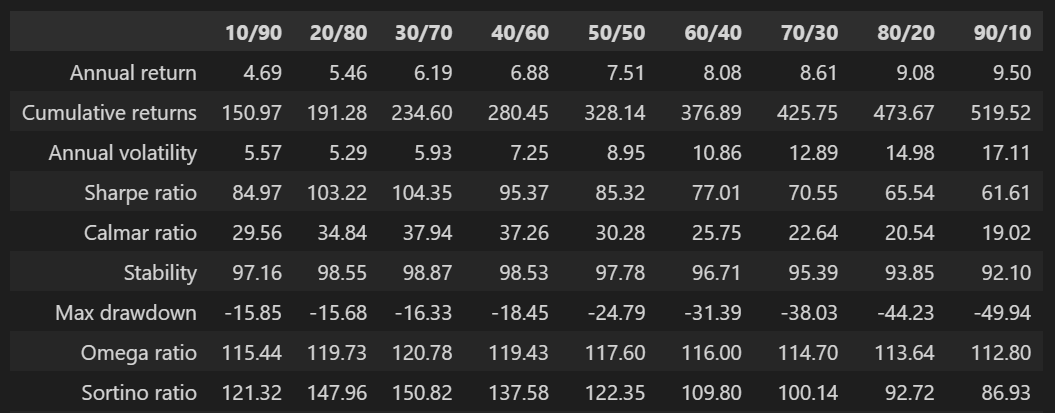
np.abs(df_stats.iloc[[0,2,3,6]]).plot.bar(figsize=(10, 5));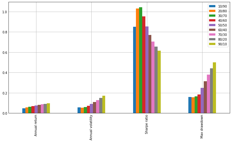
주식비중을 높일수록 연복리 수익률은 높아지지만 변동성과 MDD도 커지는 것을 확인해볼 수 있다. 샤프 비율 기준으로 가장 좋은 주식/채권 비중은 30/70으로 나타났다. 주식과 채권의 비중을 30/70으로 하면 비중이 60/40일 때보다 연복리 수익률을 2%p 정도 희생하고, MDD를 반으로 줄일 수 있게 된다.
4. 글을 마치며
이번 글에서는 60/40 포트폴리오의 백테스팅 결과를 살펴보았고, 주식과 채권 비중의 변화에 따라 달라지는 성과지표 값들을 비교해보았다. Allocate Smartly에서 사용하는 simulated data를 만들어낼 수 있으면 1970년~2001년 기간에 대한 백테스팅 결과도 비교해볼 수 있을 것 같은데, 일단 IEF의 벤치마크 인덱스 데이터를 가져오는 게 생각보다 쉽지 않았다. 이 부분은 추후에 좀 더 서칭을 해봐야 할 것 같다.
5. 참고자료
강환국, 『거인의 포트폴리오』, page2-(2021), p.155-p.161